Using CREODIAS for oil spills monitoring

Oil spills are a common cause of pollution in seas and oceans, often resulting from ship malfunctions, defective pipelines, or port accidents. Due to their harmful effects on marine life and entire ecosystems, it is crucial to detect them as early as possible to minimize damage. 

Oil spills are visible in SAR radar images. Easy access to such data is provided by the CREODIAS platform. In this project, SAR images from the Sentinel-1 sensor were used. These images were acquired in Ground Range Detected (GRD) mode with Interferometric Wide swath acquisition and VV polarization. This means that the images were obtained by transmitting the signal vertically and receiving it vertically, and then they were projected onto the WGS 84 ellipsoid. For detecting oil spills, the VV polarization yields the best results due to its enhanced ability to detect changes on the water surface. 

While object detection algorithms can be effective for detecting oil spills in satellite images, in this project a U-Net convolutional neural network was chosen for semantic segmentation. This approach produces binary masks that predict where an oil spill may be present. Such masks are easy to interpret and intuitive even for those without specialized knowledge of the characteristics of oil spills on water. 

To train the U-Net network, a dataset is required, which can be prepared by manually labeling radar images provided through CREODIAS. In this project, the training dataset consisted of fifteen Sentinel-1 SAR images and their corresponding binary masks. These images were augmented to increase the dataset's size, and then both the images and masks were divided into smaller 1024x1024 pixel chunks to preserve the spatial context of oil spills. The final step in preparing the dataset involved selecting the fragments in which oil was detected (where the masks contained pixels with a value of 1) and an equal number of fragments without oil. This resulted in a 1:1 ratio of images with oil to images without oil, and the dataset comprised 3,360 smaller images, which were then split into training and test sets in a 70:30 ratio. 

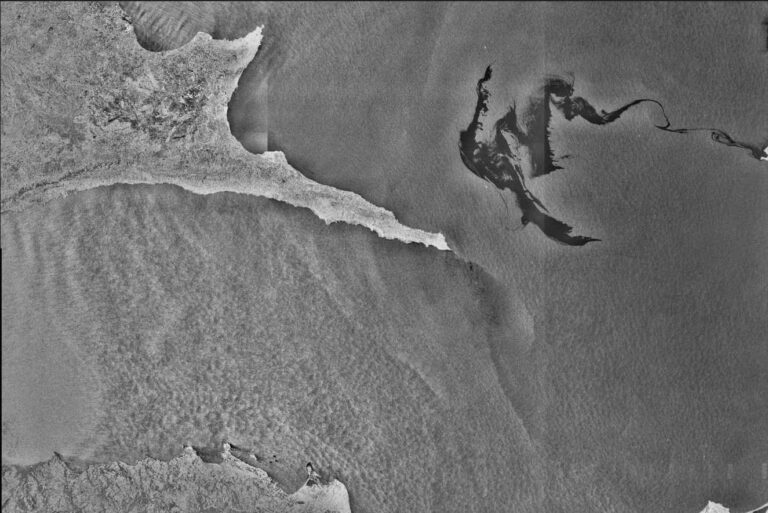
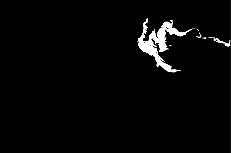
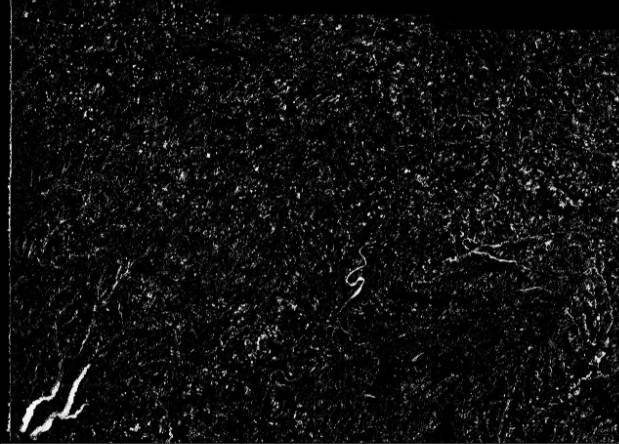
Example of processed SAR image with binary mask. Contains Copernicus Sentinel-1 modified data (2021) 

The U-Net model used in the project featured a depth of four levels, which means it contained 9 convolutional blocks with the number of filters in each layer ranging from 32 to 512. The model was trained on the prepared dataset. For applying the model to new images, the input image must be split into 1024x1024 pixels fragments. Predictions are made for these patches, and then they are combined into a single binary mask that matches the dimensions of the input image.

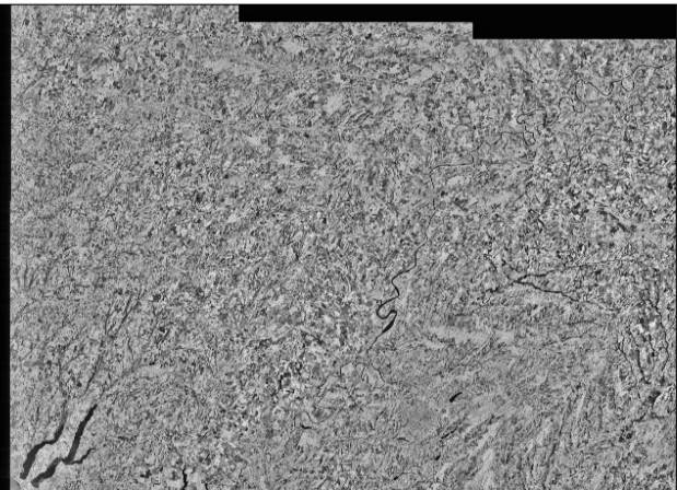
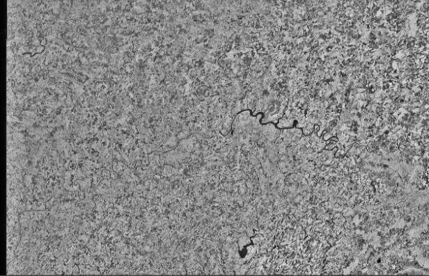
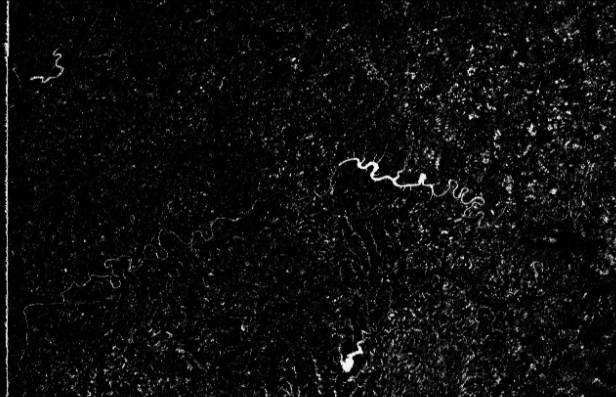
Examples of processed SAR images with predicted binary masks. Contains Copernicus Sentinel-1 modified data (2021)  

Due to the size of the dataset, the model was trained using a GPU. CREODIAS provides access to virtual machines optimized for AI and machine learning models, including those suitable for training neural networks. Once your model is trained, or a pre-trained model is used, it can be applied to predict masks on new images accessed via CREODIAS.

Step-by-step code

Step 1: Import libraries

import matplotlib.pyplot as plt
    import numpy as np
    import tensorflow as tf
    import gc
    from keras.models import load_model

Step 2: Load SAR Images from CREODIAS

In this step, the file paths containing the Sentinel-1 SAR images are extracted by specifying a date range and the coordinates of a point that must be included in the image. 

#date in format YYYY-MM-DD 

start_date='2019-08-10' 

end_date='2019-09-30' 

#coordinates of POI in WGS84 

point_x='55'  

point_y='18' 

images=get_images(start_date, end_date, point_x, point_y) #getting images from eodata that intersect point within a defined time interval 

Step 3: Load model

Specify the path to the trained model and load it.

model_path='/path/to/model'
    model=load_model(model_path)

Step 4: Predict masks for images

In this step, mask predictions are made based on the original image, which has been divided into smaller fragments. Subsequently, the smaller masks are merged into a single mask that corresponds to the dimensions of the original image.

predicted_images=predictions(images, model, crop_patch, batch_size)

Step 5: Plotting images and predicted masks

After generating the masks, they can be displayed alongside the original images.

for pred_image, image in zip(predicted_images, images):
        plt.figure(figsize=(18, 9))
        plt.subplot(121)
        plt.imshow(image, cmap='gray')
        plt.subplot(122)
        plt.imshow(pred_image, cmap='gray')
        plt.show()

The functions utilized in the code above:

def make_patches(image, patch_size):
"""
Description:
This function creates patches from the input image
Parameters:
image - input image
patch_size - width and height of patch images
"""
height, width = image.shape[:2]
patches = []
for i in range(0, height, patch_size):
    for j in range(0, width, patch_size):
        patch = image[i:i + patch_size, j:j + patch_size]
        patches.append(patch)
return patches

def combine_patches(image, patches, patch_size):
"""
Description:
This function combines small images into an image of the original size
Parameters:
image - original image
patches - patch images array
patch_size - the size of the width and height of a single patch image
"""
height=image.shape[0]
width=image.shape[1]
image=np.zeros((height, width), dtype=patches[0].dtype)
patch_idx = 0
for i in range(0, height, patch_size):
    for j in range(0, width, patch_size):
        image[i:i + patch_size, j:j + patch_size] = patches[patch_idx]
        patch_idx += 1
return image

def predictions(images, model, crop_patch, batch_size):
"""
Description:
This function predicts masks for the input images
Parameters:
images - array of input images
model - U-net model
crop_patch - width and height of a patch images
batch_size - number of batch in a model
"""
predicted_images=[]
for image in images:
    image_patches=make_patches(image, crop_patch) #making patches from the image
    image_patches=np.array(image_patches)
    image_patches=np.expand_dims(image_patches, axis=-1) #adding another dimension
    img_predict=model.predict(image_patches, batch_size=batch_size) #predicting a mask for each image
    img_predict=np.squeeze(img_predict, axis=-1) #removal of the added dimension
    reconstructed=combine_patches(image, img_predict, crop_patch) #combinig patches into an image
    predicted_images.append(reconstructed)
    del image_patches, img_predict, reconstructed
    gc.collect()
return predicted_images

def get_images(start_date, end_date, point_x, point_y):
"""
Description:
This function gets images that intersect point within a defined time interval
Parameters:
start_date - date in format YYYY-MM-DD
end_date - date in format YYYY-MM-DD
point_x - X-coordinates of POI in WGS84
point_y - Y-coordinates of POI in WGS84
"""
images=[]
crop_patch=1024
k=0
n=0
kernel_size=25
sap_filtr=13
url=f'https://datahub.creodias.eu/odata/v1/Products?\$filter=((ContentDate/Start%20ge%20{start_date}T00:00:00.000Z%20and%20ContentDate/Start%20le%20{end_date}T23:59:59.999Z)%20and%20(Online%20eq%20true)%20and%20(OData.CSC.Intersects(Footprint=geography%27SRID=4326;POINT%20({point_x}%20{point_y})%27))%20and%20(((((Collection/Name%20eq%20%27SENTINEL-1%27)%20and%20(((Attributes/OData.CSC.StringAttribute/any(i0:i0/Name%20eq%20%27productType%27%20and%20i0/Value%20eq%20%27GRD%27)))))))))&\$expand=Attributes&\$expand=Assets&\$orderby=ContentDate/Start%20asc&\$top=20\'
products=json.loads(requests.get(url).text)
path_list=[]
for item in products[\'value\']:
path_list.append(item[\'S3Path\'])
del url
del products
for dir_path in path_list:
    matching_dir=glob.glob(os.path.join(dir_path, 'measurement'))
    for dir in matching_dir:
        for root, dirs, files in os.walk(dir):
            for file in files:
                file_path=None
                if file.endswith(\'001.tiff\'): #only first tiff file
                    file_path=glob.glob(os.path.join(dir, file))[0] #importing path
                if file_path:
                    '''operations on the original image'''
                    image=cv2.imread(file_path, cv2.IMREAD_UNCHANGED)
                    x_start, y_start=k*crop_patch, n*crop_patch #cooridnates of upper left corner
                    x_end, y_end=(image.shape[1]//crop_patch)*crop_patch, (image.shape[0]//crop_patch *crop_patch #coordinates of bottom right corner
                    image=image[y_start:y_end, x_start:x_end] #image cropping
                    del x_start, y_start, x_end, y_end
                    '''image normalization to grayscale (0-255) and operations on it'''
                    scaled=scale_array(image) #image scaling
                    scaled = cv2.normalize(scaled, None, 0, 255,
                    cv2.NORM_MINMAX).astype(np.uint8) #conversion from uint16 to uint8
                    del image
                    '''increase photo contrast'''
                    clahe = cv2.createCLAHE(clipLimit=4.0, tileGridSize=(kernel_size, kernel_size)) #histogram equalization
                    clahe_scaled = clahe.apply(scaled)
                    del scaled
                    '''denoising an image'''
                    median_image=cv2.medianBlur(clahe_scaled, sap_filtr) #salt and pepper noise filtering
                    del clahe_scaled
                    images.append(median_image)
return images