


Satellite-based wildfire monitoring in California using EO data on CREODIAS
California has recently experienced a series of severe wildfires, exacerbated by climate change. Rising temperatures, prolonged droughts, and strong winds create an environment highly susceptible to fire outbreaks (Soulé and Knapp, 2024). Effective wildfire monitoring is crucial for disaster management and damage mitigation (Boroujeni et al., 2024).
In addressing this complex challenge, the EOData repository on the CREODIAS platform has been utilized to provide high-resolution satellite imagery, enabling rapid fire detection and damage assessment. This is made possible by the CREODIAS platform, which provides Copernicus Sentinel-2 data captured at various wavelengths, ranging from 490 nm (blue) to 2190 nm (SWIR 2).
The shortest wavelength (490 nm) is useful for distinguishing between soil, vegetation, and man-made structures. After a fire, it helps identify burned areas when combined with other bands, particularly in regions with significant post-fire contrast. On the other hand, the longest wavelength (2190 nm) aids in detecting burned areas and assessing post-fire conditions, especially by monitoring moisture content in soil and vegetation.
The wavelengths within this range are valuable for mapping burned areas, assessing fire severity and vegetation loss, detecting vegetation changes, supporting burned-area mapping, monitoring recovery, and differentiating vegetation types to evaluate fire impact.
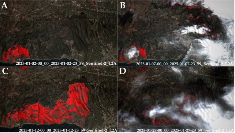
Several images illustrating the results of using the EOData repository for wildfire monitoring in California are shown in Figure 1.
It is worth mentioning that the EOData repository from CREODIAS is not only useful for immediate detection and response but also plays a vital role in post-fire analysis. Satellite imagery can be used to assess the extent of burned areas, monitor vegetation regeneration, and analyze the long-term environmental effects of fire, such as soil erosion, water quality, and biodiversity loss. When combined with climate and weather forecasting models, this data also helps researchers predict fire-prone areas and better understand the relationships between environmental conditions, land use, and fire risk.
The code presented below is designed for the visualization of areas experiencing active wildfires. It leverages satellite imagery from the Sentinel-2 mission to accurately identify and illustrate burned regions.
Step-by-step code walkthrough
Step 1: Accessing the CREODIAS Platform
To initiate work with satellite imagery from the CREODIAS platform, it is necessary to establish an account. Comprehensive information regarding the registration process can be found at the following link: https://creodias.eu/. Users have the option to acquire data through OpenEO, S3, or the RESTO API, depending on their specific requirements.
Step 2: Define the Area of Interest and Temporal Range
It is imperative to specify the bounding box (BBOX) that delineates the area of interest, as well as the temporal range for the satellite data retrieval. This ensures that the selected area and dates correspond with relevant wildfire events for effective monitoring and analysis.
Step 3: Import Required Libraries
import os
import numpy as np
import rasterio
from rasterio.enums import Resampling
import matplotlib.pyplot as plt
Step 4: Specify the Directory for Sentinel-2 Data
Specify the directory where the Sentinel-2 data is stored. Adjust the path according to your data structure.
#Path to the directory containing Sentinel-2 data
img_data_dir = "Sentinel2_data/"
Step 5: Identify Sentinel-2 Band Files
In this step, we search for specific JP2 files that correspond to different bands of Sentinel-2 data. It fills the band_files dictionary with the file paths of the required bands. Search for JP2 files corresponding to the necessary Sentinel-2 spectral bands.
band_files = {band: None for band in ["B02", "B03", "B04", "B08", "B11", "B12"]}

for filename in os.listdir(img_data_dir):
    for band in band_files.keys():
        if band in filename and filename.endswith(".jp2"):
            band_files[band] = os.path.join(img_data_dir, filename)
Step 6: Check for Missing Bands
This step ensures that all required bands are found. If any bands are missing, a `FileNotFoundError` is raised.
missing_bands = [band for band, path in band_files.items() if path is None]
if missing_bands:
    raise FileNotFoundError(f"Missing bands: {', '.join(missing_bands)}")
Step 7: Load Bands and Rescale to 10m Resolution
We load the required bands and rescale them to a common resolution (e.g., 10m).
bands = {}
with rasterio.open(band_files["B02"]) as src:
    ref_shape = src.shape  # Target resolution (e.g., 10m)

for band, filepath in band_files.items():
    with rasterio.open(filepath) as src:
        bands[band] = src.read(1, out_shape=ref_shape, resampling=Resampling.bilinear).astype(np.float32)
Step 8: Normalize Band Values
In this step, each band is normalized to a range of 0 to 1 for further processing.
#Normalize band values (Sentinel-2 often has values ranging from 0 to 10000)
for band in bands:
    bands[band] /= np.max(bands[band])
Step 9: Calculate Indices
We calculate various indices such as NDWI (Normalized Difference Water Index), NDVI (Normalized Difference Vegetation Index), and a Burned Area Index.
def index(a, b):
    eps = 1e-6  # Avoid division by zero
    return (a - b) / (a + b + eps)

NDWI = index(bands["B03"], bands["B08"])  # Normalized Difference Water Index
NDVI = index(bands["B08"], bands["B04"])  # Normalized Difference Vegetation Index
INDEX = index(bands["B11"], bands["B12"]) + bands["B08"]  # Burned Area Index
Step 10: Create a Burned Area Mask
We create an RGB image to visualize the data. This step also prepares for further analysis of burned areas.
rgb_image = np.zeros((ref_shape[0], ref_shape[1], 4)) # Initialize RGB image with 4 bands (including alpha)Step 11: Apply Thresholds for Burned Area Detection
We apply thresholds to identify burned areas in the image.
for i in range(ref_shape[0]):
    for j in range(ref_shape[1]):
        if (INDEX[i, j] > 0.1) or (bands["B02"][i, j] > 0.1) or (bands["B11"][i, j] < 0.1) or (NDVI[i, j] > 0.3) or (NDWI[i, j] > 0.1):
            rgb_image[i, j, 0] = 2.5 * bands["B04"][i, j]  # Red channel
            rgb_image[i, j, 1] = 2.5 * bands["B03"][i, j]  # Green channel
            rgb_image[i, j, 2] = 2.5 * bands["B02"][i, j]  # Blue channel
            rgb_image[i, j, 3] = 1  # Alpha channel (visible)
        else:
            rgb_image[i, j, 0] = 1  # Red channel
            rgb_image[i, j, 1] = 0  # Green channel
            rgb_image[i, j, 2] = 0  # Blue channel
            rgb_image[i, j, 3] = 1  # Alpha channel (visible)
Step 12: Clip Values to Range [0, 1]
In this step, the values of the RGB image are clipped to ensure they fall within the range [0, 1].
rgb_image = np.clip(rgb_image, 0, 1)Step 13: Convert to 8-bit for Display
Convert the RGB image to 8-bit format for display.
rgb_image_display = (rgb_image[:, :, :3] * 255).astype(np.uint8)Step 14: Display the Image
Finally, we display the RGB image to visualize the burned areas. The image is shown with the specified title and axes are turned off for a cleaner view.
plt.figure(figsize=(10, 8))
plt.imshow(rgb_image_display)
plt.title("Burned Area Detection")
plt.axis("off")  # Turn off axis
plt.show()
References:
Boroujeni, S.P.H., Razi, A., Khoshdel, S., Afghah, F., Coen, J.L., O’Neill, L., Fule, P., Watts, A., Kokolakis, N.-M.T., Vamvoudakis, K.G., 2024. A comprehensive survey of research towards AI-enabled unmanned aerial systems in pre-, active-, and post-wildfire management. Information Fusion 102369.
Sinergise, S.-H. by, n.d. Sentinel-2 Bands [WWW Document]. Sentinel Hub custom scripts. URL https://custom-scripts.sentinel-hub.com/custom-scripts/sentinel-2/bands/ (accessed 1.31.25).
Soulé, P.T., Knapp, P.A., 2024. The evolution of “Hot” droughts in Southern California, USA from the 20th to the 21st century. Journal of Arid Environments 220, 105118.
Author: Dr. Eng. Ewa Panek-Chwastyk, Remote Sensing Centre, Institute of Geodesy and Cartography, Warsaw, Poland
Read also:
- Using CREODIAS for oil spills monitoring
- 2025 - a year of EO embeddings?
- Monitoring inland water quality in Poland using Python and Sentinel-2 satellite imagery
- Monitoring Vegetation Using Sentinel-1 Data: the RVI Calculator
- Potential of the Copernicus data in flood prediction and monitoring
Check out more articles in the Use cases section of the Knowledgebase.