Using CREODIAS for water quality monitoring 

Author: Bartosz Skóra, Data Science (Participant of the Internship Programme at CloudFerro), Contact: bskora@cloudferro.com 

Water quality is essential for ecosystem health, drinking water safety, and the sustainable use of aquatic resources. Monitoring parameters such as turbidity, chlorophyll concentration, and dissolved organic matter helps detect pollution, eutrophication, and seasonal dynamics. Traditional in-situ measurements are accurate but limited in coverage. With the use of Copernicus Sentinel satellite data, we can monitor large water bodies efficiently. Easy access to such data is provided by the CREODIAS platform. 

This study focuses on Manila Bay, a critical coastal region in the Philippines that supports fisheries, trade, and the livelihoods of millions of people in Metro Manila. For this analysis, Sentinel-2 imagery acquired on 01/06/2025 was used. The bay faces significant environmental challenges, including nutrient loading from rivers, untreated wastewater discharge, sedimentation, and harmful algal blooms. Satellite-based monitoring provides valuable insight into these issues and complements traditional water sampling. 

All calculations and processing steps were performed directly in the CREODIAS cloud infrastructure, ensuring efficient access to large EO datasets. Sentinel-2 Level-2A surface reflectance data was accessed via EODATA storage mounted directly on CloudFerro virtual machines available on CREODIAS, which eliminated the need to download the data. Several spectral indices related to water quality were derived from 20 m resolution bands:

Indices were calculated using empirical models from previous studies [1,2]. It is important to note that while these indices provide useful relative patterns, they cannot directly replace in-situ measurements. Without calibration against ground-truth data, values remain approximate and should be interpreted with caution. 

Manila Bay is a semi-enclosed coastal system with limited water exchange, making it particularly vulnerable to pollution and eutrophication. The bay supports important economic activities such as fishing, aquaculture, and shipping, but it also faces a lot of challenges related to water quality. Key challenges include:

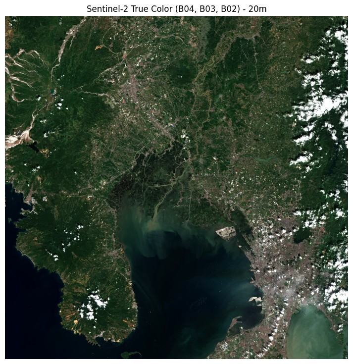
The Sentinel-2 RGB composite (bands B04, B03, B02) provides a natural color view of Manila Bay, highlighting the contrast between urbanized coastal areas and surrounding vegetation. 

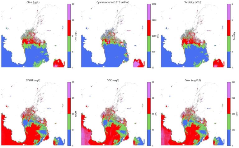
Based on the resulting maps we observe high concentration of Chl-a in the northern part of the bay and highest close o river mouths indicating eutrophication hot-spots and potential algal blooms. Central Bay waters show lower concentration, reflecting clearer conditions. Cyanobacteria concentrations follow a similar pattern to Chl-a, which highlights the risk of harmful algal bloom likely driven by nutrient-rich river discharges. Turbidity also peaks along the northern coast, while offshore waters remain relatively clear. CDOM and DOC indices have very close concentration highest in offshore water and very close to shore with a transitional zone in between that appears relatively clearer. The Color index mirrors these patterns, which is expected since CDOM and DOC strongly influence the visible color of water, making it appear darker where concentrations are higher. 

Satellite monitoring, as demonstrated in this study, allows for continuous large-scale assessment of these dynamics, supporting sustainable management and restoration efforts. However, integration with ground-based in-situ measurements remains essential for validation and accurate quantification. 

Step by step code

Step 1: Import libraries

import requests
import json
import pandas as pd
import numpy as np
import matplotlib.pyplot as plt
import os
import boto3
import rasterio
import matplotlib.colors as mcolors

Step 2: Connect to eodata s3 bucket

# Enter your eodata credentials here:
access_key = ''
secret_key = ''
host = 'https://eodata.cloudferro.com'

# Initialize S3 resource
s3 = boto3.resource(
    's3',
    aws_access_key_id=access_key,
    aws_secret_access_key=secret_key,
    endpoint_url=host,
)

# Verify connection by accessing the 'eodata' bucket
bucket_name = 'eodata'
try:
    bucket = s3.Bucket(bucket_name)
    # Check if the bucket is accessible by listing its contents
    objects = list(bucket.objects.limit(1)) # Limit to 1 object for testing
    if objects:
        print(f"Connection to bucket '{bucket_name}' successful. Objects found.")
    else:
        print(f"Connection to bucket '{bucket_name}' successful, but no objects found.")
except Exception as e:
    print(f"Connection to bucket '{bucket_name}' failed:", e)

Step 3: Create a search query for Manila Bay

# Search parameters: Sentinel-2 L2A over Manila Bay
catalogue_odata_url = "https://datahub.creodias.eu/odata/v1"
collection_name = "SENTINEL-2"
product_type = "S2MSI2A"  # Level-2A (surface reflectance)

# AOI: Manila Bay
aoi = "POLYGON((121.05 14.65, 121.50 14.65, 121.50 14.15, 121.05 14.15, 121.05 14.65))"

# Time window: wide window to get more scenes
search_period_start = "2024-01-01T00:00:00.000Z"
search_period_end = "2025-08-26T23:59:59.000Z"

# Optional: Cloud coverage <10% for clearer images
cloud_cover_max = 10.0

search_query = (
    f"{catalogue_odata_url}/Products?"
    f"$filter=Collection/Name eq '{collection_name}' "
    f"and Attributes/OData.CSC.StringAttribute/any(att:att/Name eq 'productType' "
    f"and att/OData.CSC.StringAttribute/Value eq '{product_type}') "
    f"and Attributes/OData.CSC.DoubleAttribute/any(att:att/Name eq 'cloudCover' "
    f"and att/OData.CSC.DoubleAttribute/Value lt {cloud_cover_max}) "
    f"and OData.CSC.Intersects(area=geography'SRID=4326;{aoi}') "
    f"and ContentDate/Start gt {search_period_start} "
    f"and ContentDate/Start lt {search_period_end}"
    f"&$top=1000"
)

print(search_query)

Step 4: Check products and print paths to eodata folder

response = requests.get(search_query).json()
result = pd.DataFrame.from_dict(response["value"])
print(f'Number of products which meets query filters: {len(result)}')

products = json.loads(requests.get(search_query).text)
path_list = []
for item in products['value']:
    path_list.append(item['S3Path'])

path_list

Step 5: Load bands and normalize

output_dir = path_list[x]

def find_and_load_s2_bands_20m(safe_folder, bands):
    """
    Find and load Sentinel-2 bands at 20m resolution (JP2 files) inside a .SAFE folder.
    Returns a dict {band_name: array}.
    """
    band_data = {}

    for root, dirs, files in os.walk(safe_folder):
        if "R20m" in root:  # only look into the 20m folder
            for file_name in files:
                if file_name.lower().endswith(".jp2"):
                    for band in bands:
                        if f"{band}.jp2" in file_name or f"_{band}_" in file_name:
                            path = os.path.join(root, file_name)
                            with rasterio.open(path) as src:
                                band_data[band] = src.read(1)
                            print(f"Loaded {band}: {path}")
    return band_data

# Example usage
bands_needed = ("B01","B02","B03","B04","SCL")
s2_bands_20m = find_and_load_s2_bands_20m(output_dir, bands_needed)

# Access arrays directly
b01 = s2_bands_20m.get("B01")
b02 = s2_bands_20m.get("B02")
b03 = s2_bands_20m.get("B03")
b04 = s2_bands_20m.get("B04")
scl = s2_bands_20m.get("SCL")

print("Bands loaded:", list(s2_bands_20m.keys()))

# Band normalization
b01 = b01 / 10000.0
b02 = b02 / 10000.0
b03 = b03 / 10000.0
b04 = b04 / 10000.0

Step 6: Create water mask from SCL

# Water pixels are classified with value 6 in the SCL band
water_mask = (scl == 6)

# Print number of water pixels
print("Water pixels:", int(water_mask.sum()))

Step 7: Calculate indices and plot

# Formulas for water quality parameters
chl_a = 4.26 * np.power((b03 / b01), 3.94)
cya = 115530.31 * np.power(((b03 * b04) / b02), 2.38)
turb = 8.93 * (b03 / b01) - 6.39
cdom = 537 * np.exp(-2.93 * (b03 / b04))
doc = 432 * np.exp(-2.24 * (b03 / b04))
color = 25366 * np.exp(-4.53 * (b03 / b04))

# Clip values (remove outliers)
chl_a = np.clip(chl_a, 0, np.nanpercentile(chl_a, 95))
cya = np.clip(cya, 0, np.nanpercentile(cya, 95))
cdom = np.clip(cdom, 0, np.nanpercentile(cdom, 95))
doc = np.clip(doc, 0, np.nanpercentile(doc, 95))
color = np.clip(color, 0, np.nanpercentile(color, 95))
turb = np.clip(turb, 0, np.nanpercentile(turb, 95))

# Apply water mask
chl_a = np.where(water_mask, chl_a, np.nan)
cya = np.where(water_mask, cya, np.nan)
turb = np.where(water_mask, turb, np.nan)
cdom = np.where(water_mask, cdom, np.nan)
doc = np.where(water_mask, doc, np.nan)
color = np.where(water_mask, color, np.nan)

# Custom scales
scaleChl_a = [0, 5, 8, 11, 16]
scaleCya = [12, 900, 1300, 2100, 5200]
scaleTurb = [0, 3, 4, 5, 6]
scaleCDOM = [0, 17, 20, 25, 35]
scaleDOC = [0, 30, 35, 40, 50]
scaleColor = [0, 120, 160, 210, 350]

# Norms
norm_chl = mcolors.BoundaryNorm(scaleChl_a, custom_cmap.N)
norm_cya = mcolors.BoundaryNorm(scaleCya, custom_cmap.N)
norm_turb = mcolors.BoundaryNorm(scaleTurb, custom_cmap.N)
norm_cdom = mcolors.BoundaryNorm(scaleCDOM, custom_cmap.N)
norm_doc = mcolors.BoundaryNorm(scaleDOC, custom_cmap.N)
norm_col = mcolors.BoundaryNorm(scaleColor, custom_cmap.N)

# Plot results
fig, axs = plt.subplots(2, 3, figsize=(18, 12))
im1 = axs[0,0].imshow(chl_a, cmap=custom_cmap, norm=norm_chl); axs[0,0].set_title("Chl-a (µg/L)")
im2 = axs[0,1].imshow(cya, cmap=custom_cmap, norm=norm_cya); axs[0,1].set_title("Cyanobacteria (10^3 cell/ml)")
im3 = axs[0,2].imshow(turb, cmap=custom_cmap, norm=norm_turb); axs[0,2].set_title("Turbidity (NTU)")
im4 = axs[1,0].imshow(cdom, cmap=custom_cmap, norm=norm_cdom); axs[1,0].set_title("CDOM (mg/l)")
im5 = axs[1,1].imshow(doc, cmap=custom_cmap, norm=norm_doc); axs[1,1].set_title("DOC (mg/l)")
im6 = axs[1,2].imshow(color, cmap=custom_cmap, norm=norm_col); axs[1,2].set_title("Color (mg.Pt/l)")

for ax, im, label in zip(axs.flat,
    [im1, im2, im3, im4, im5, im6],
    ["Chl-a (µg/L)", "Cya", "Turbidity", "CDOM", "DOC", "Color"]):
    plt.colorbar(im, ax=ax, fraction=0.046, pad=0.04, label=label)
    ax.axis("off")

plt.tight_layout()
plt.show()

Step 8: Optionally plot RGB image

# Stack into RGB
rgb = np.dstack([b04, b03, b02])

# Stretch between 2nd–98th percentile
rgb_min, rgb_max = np.percentile(rgb, (2, 98))
rgb_stretched = np.clip((rgb - rgb_min) / (rgb_max - rgb_min), 0, 1)

# Plot
plt.figure(figsize=(9,9))
plt.imshow(rgb_stretched)
plt.title("Sentinel-2 True Color (B04, B03, B02) - 20m")
plt.axis("off")
plt.show()

---

References:

[1] K. Toming, T. Kutser, A. Laas, M. Sepp, B. Paavel, and T. Nıges, First Experiences in Mapping Lake Water Quality Parameters with Sentinel-2 MSI Imagery, Remote Sens., vol. 8, no. 8, p. 640, Aug. 2016. 

[2] M. Potes et al., Use of Sentinel 2-MSI for water quality monitoring at Alqueva reservoir, Portugal, Proc. Int. Assoc. Hydrol. Sci., vol. 380, pp. 73ñ79, Dec. 2018.