Sen2VHR-35K: 10 m-to-2 m Super-Resolution on CREODIAS

Tom Aucler, University of Ljubljana, Faculty of Computer and Information Science 

Introduction

Sentinel-2 provides multispectral Earth observation imagery with broad geographic coverage and frequent revisit capability. However, its commonly used visible and near-infrared bands have a spatial resolution of 10 m, which limits the interpretation of small objects, narrow infrastructure, heterogeneous urban structures and fine land-cover patterns.

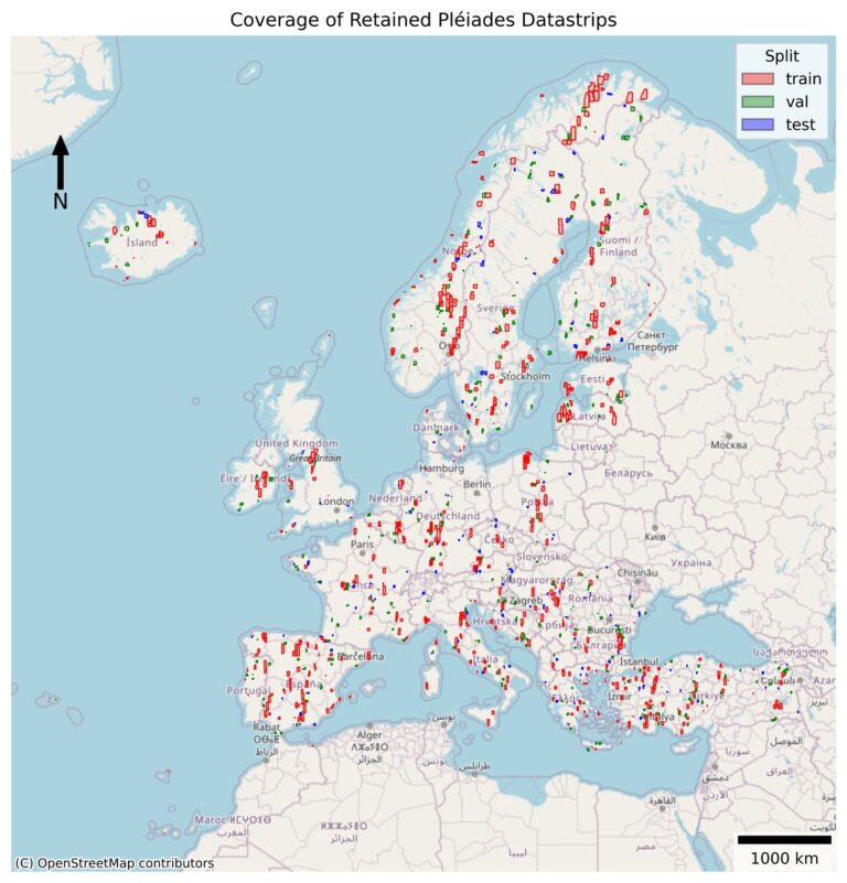
The presented use case investigates whether a deep-learning super-resolution model can reconstruct four-band imagery (red, green, blue and near-infrared) from 10 m Sentinel-2 inputs at a target ground sampling distance of 2 m. The work is based on the Sen2VHR-35K dataset, consisting of spatially paired Sentinel-2 and Pléiades very-high-resolution image patches.

Training a generative super-resolution network on tens of thousands of multispectral image pairs requires substantial GPU memory, storage throughput and processing capacity. The CREODIAS platform was used to provide the cloud infrastructure required for dataset handling, model training, inference and systematic checkpoint evaluation.

The implementation was deployed on a CREODIAS virtual machine equipped with an NVIDIA H100 NVL GPU, approximately 96 GB of GPU memory and 220 GB of system memory. This configuration enabled training with 256 × 256-pixel four-band Sentinel-2 inputs and corresponding 1280 × 1280-pixel four-band VHR targets.

The generated images can support visual interpretation and downstream analysis, but they must not be treated as equivalent to directly acquired 2 m imagery. Super-resolution models may introduce spatial details that are plausible but not present in the original observation. For this reason, the implementation includes an auxiliary confidence layer intended to indicate where reconstruction errors are expected to be higher.

This work was carried out as part of the first author's doctoral research, during which the Sen2VHR-35K dataset was developed. The dataset provides the paired Sentinel-2 and Pléiades imagery used to train and evaluate the proposed super-resolution model.

Brief solution summary

The solution implements a modified Enhanced Super-Resolution Generative Adversarial Network, or ESRGAN, for five-fold multispectral super-resolution. 

The main workflow comprises: 

1. preparation of paired Sentinel-2 and Pléiades image patches; 
2. division of the dataset into training, validation and test subsets at datastrip level; 
3. standardisation of each Sentinel-2 input patch; 
4. generator warm-up using pixel-wise mean squared error; 
5. adversarial training of the generator and discriminator; 
6. simultaneous learning of a per-pixel expected-error layer; 
7. checkpoint-based validation and model comparison; 
8. folder-based inference producing four-band super-resolved GeoTIFFs and confidence layers. 

The model uses: 

• four input channels: red, green, blue and near-infrared; 
• four super-resolved output channels; 
• a five-fold spatial enlargement from 256 × 256 to 1280 × 1280 pixels; 
• 23 residual-in-residual dense blocks; 
• 64 backbone feature channels; 
• an auxiliary one-channel expected-MAE output head; 
• bfloat16 mixed-precision computation; 
• Adam optimisation; 
• a 10-epoch reconstruction warm-up; 
• adversarial training for the remaining epochs; 
• MultiStep learning-rate scheduling with milestone epochs at 75, 125 and 175 (decay factor of 0.5); 
• 200 total training epochs. 

More information about the model architecture is available in the original ESRGAN paper: Wang, X.; Yu, K.; Wu, S.; Gu, J.; Liu, Y.; Dong, C.; Qiao, Y.; Loy, C.C. ESRGAN: Enhanced Super-Resolution Generative Adversarial Networks. In Proceedings of the European Conference on Computer Vision Workshops, 2018. 

Results 

The ESRGAN baseline was evaluated on the test split of the dataset using Peak Signal-to-Noise Ratio (PSNR), Structural Similarity Index (SSIM), Spectral Angle Mapper (SAM), and Learned Perceptual Image Patch Similarity (LPIPS). 

The selected metrics capture complementary aspects of reconstruction quality. PSNR380 

measures pixel-wise reconstruction fidelity by quantifying the difference between the super-resolved and reference pixel values; higher values indicate that reconstructed pixel values are closer to the target image. SSIM evaluates structural similarity by comparing local patterns of luminance, contrast, and spatial structure, making it sensitive to the preservation of edges, textures, and object shapes; higher values indicate better structural preservation. SAM measures the angle between predicted and reference spectral vectors at each pixel, and thus evaluates how well the spectral relationships between bands are preserved independently of overall brightness; lower values indicate better spectral consistency. LPIPS estimates perceptual similarity using deep feature representations extracted from a pretrained neural network and is designed to better reflect human visual perception of image quality; lower values indicate that reconstructed images appear perceptually closer to the reference images. 

The results are presented in the following table, together with a bicubic interpolation baseline for reference. 

Metric	ESRGAN	Bicubic	∆
PSNR (dB) ↑	21.55	19.74	+1.81
SSIM ↑	0.658	0.675	-0.017
SAM (deg) ↓	9.79	10.92	-1.13
LPIPS ↓	0.361	0.584	-0.224

Table: Baseline super-resolution performance on the test split. ∆ denotes the difference between ESRGAN and bicubic interpolation. Arrows indicate whether higher (↑) or lower (↓) values correspond to better performance. 

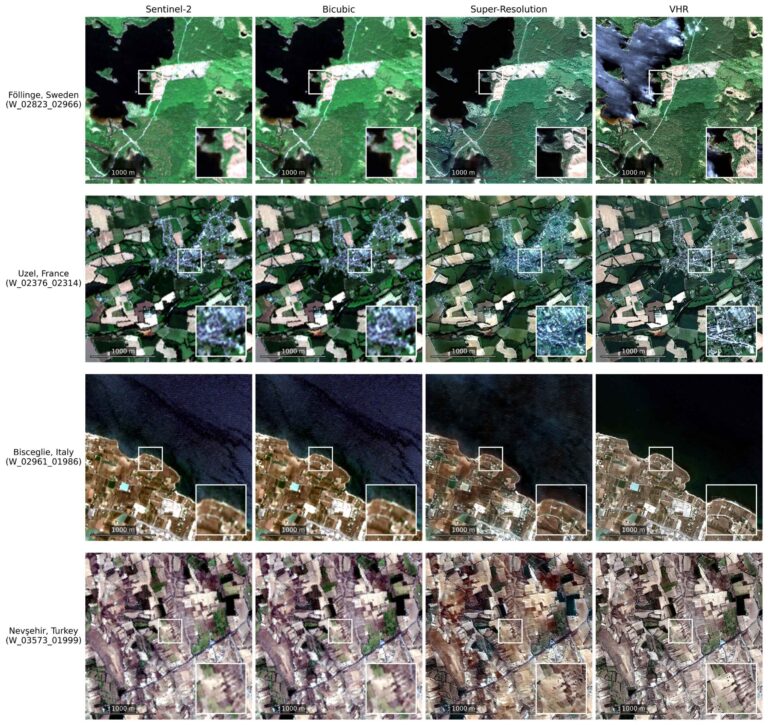
The ESRGAN model improves pixel-wise fidelity, achieving a gain of +1.81 dB in PSNR over bicubic interpolation. Spectral consistency is also enhanced, as indicated by a reduction of the mean spectral angle (SAM) by 1.13°.  

In terms of perceptual quality, ESRGAN attains a substantially lower LPIPS score, reflecting improved texture realism and sharper spatial details compared to bicubic interpolation. 

A slight decrease in SSIM is observed. This behaviour is consistent with generative super-resolution methods, which prioritise perceptual realism and high-frequency detail reconstruction over pixel-wise fidelity. In contrast, PSNR- and SSIM-oriented approaches tend to favour smoother solutions and may suppress high-frequency content, despite achieving higher similarity scores.  

Overall, these results demonstrate that the dataset supports stable supervised training and enables meaningful reconstruction improvements across both spectral and perceptual metrics. 

Step-by-step solution walkthrough 

1. Provision the CREODIAS virtual machine

A GPU-enabled Ubuntu virtual machine was provisioned through CREODIAS. CREODIAS offers configurable cloud resources and Earth-observation-oriented processing environments close to relevant EO data repositories.

The GPU configuration was verified using:

nvidia-smi

The Python environment was then created:

python3 -m venv .venv
source .venv/bin/activate

python -m pip install --upgrade pip setuptools wheel
pip install -r requirements.txt

An example dependency file is:

torch
torchvision
numpy
scipy
rasterio
geopandas
pandas
matplotlib
contextily
tqdm
scikit-image
lpips
pillow

Training was executed within tmux so that it could continue if the SSH connection was interrupted:

tmux new -s sr-training
source .venv/bin/activate
python train.py

2. Prepare paired image patches

Each dataset item consists of:

Sentinel-2 input:  4 × 256 × 256 pixels
Pléiades target:   4 × 1280 × 1280 pixels
Scale factor:      5
Band order:        Red, Green, Blue, NIR

The files are organised as:

data/
├── train/
│   ├── s2/
│   └── vhr/
├── val/
│   ├── s2/
│   └── vhr/
└── test/
    ├── s2/
    └── vhr/

The split is assigned at datastrip level rather than patch level. This prevents patches from the same Pléiades acquisition from appearing in different subsets and reduces spatial and temporal leakage.

3. Apply the same preprocessing in all phases

During training, each Sentinel-2 patch is standardised using a global z-score calculated over all bands and pixels:

import scipy.stats

s2_img = scipy.stats.zscore(s2_img, axis=None)

The same transformation must be applied during validation, test evaluation and operational inference:

import numpy as np

def zscore_global(
    image: np.ndarray,
    eps: float = 1e-6,
) -> np.ndarray:
    mean = float(image.mean())
    std = float(image.std())

    if std < eps:
        raise ValueError("Cannot standardise an image with near-zero variance.")

    return ((image - mean) / std).astype(np.float32)

Using different preprocessing during inference would shift the input distribution relative to training and could severely degrade the generated output.

4. Construct the modified ESRGAN generator

The backbone contains 23 RRDB blocks and retains the defined architecture. A second output head predicts expected MAE.

class Generator(nn.Module):

    def __init__(self, in_nc=4, out_nc=4, nf=64, nb=23, gc=32, scale=5, with_confidence=True, ):

        super().init()
        self.scale = scale
        self.with_confidence = with_confidence

        self.conv_first = nn.Conv2d(in_nc, nf, 3, 1, 1)
        self.RRDB_trunk = self.make_layer(
            lambda: RRDB(nf, gc),
            nb,
        )
        self.trunk_conv = nn.Conv2d(nf, nf, 3, 1, 1)

        self.upconv = nn.Conv2d(nf, nf, 3, 1, 1)
        self.HRconv = nn.Conv2d(nf, nf, 3, 1, 1)

        self.conv_last_sr = nn.Conv2d(nf, out_nc, 3, 1, 1)
        self.conv_last_mae = nn.Conv2d(nf, 1, 3, 1, 1)

        self.lrelu = nn.LeakyReLU(0.2, inplace=True)

    def forward(self, x):
        features = self.conv_first(x)
        trunk = self.trunk_conv(self.RRDB_trunk(features))
        features = features + trunk

        height, width = x.shape[-2:]
        features = F.interpolate(
            features,
            size=(height * self.scale, width * self.scale),
            mode="nearest",
        )

        features = self.lrelu(self.upconv(features))
        features = self.lrelu(self.HRconv(features))

        sr = self.conv_last_sr(features)
        predicted_mae = F.softplus(self.conv_last_mae(features))

        return sr, predicted_mae

The softplus activation constrains the predicted error to non-negative values.

5. Perform generator warm-up

For the first 10 epochs, only the generator is trained. The discriminator is not updated, and the generator objective consists solely of MSE reconstruction loss:

warmup = epoch < cfg.WARMUP_EPOCHS

with autocast("cuda", dtype=torch.bfloat16):
    generated_hr, predicted_mae = generator(lr_images)

    if warmup:
        generator_loss = mse_loss(generated_hr, hr_images)

This stage teaches the generator an initial reconstruction mapping before adversarial gradients are introduced.

6. Enable adversarial and confidence training

After warm-up, the generator loss combines reconstruction, adversarial and confidence terms:

[Equation]

The corresponding implementation is:

with autocast("cuda", dtype=torch.bfloat16):
    generated_hr, predicted_mae = generator(lr_images)

    fake_prediction = discriminator(generated_hr)
    valid_labels = torch.ones_like(fake_prediction)

    pixel_loss = l1_loss(generated_hr, hr_images)
    adversarial_loss = gan_loss(fake_prediction, valid_labels)

    actual_mae = torch.abs(
        generated_hr - hr_images
    ).mean(dim=1, keepdim=True)

    confidence_loss = l1_loss(
        predicted_mae,
        actual_mae.detach(),
    )

    generator_loss = (
        pixel_loss
        + cfg.LAMBDA_ADV * adversarial_loss
        + cfg.LAMBDA_CONF * confidence_loss
    )

The detach() operation is important. It prevents the confidence target from modifying the super-resolution output through the target calculation.

The discriminator is then trained on real and generated VHR images:

with autocast("cuda", dtype=torch.bfloat16):
    real_prediction = discriminator(hr_images)
    fake_prediction = discriminator(generated_hr.detach())

    real_loss = gan_loss(
        real_prediction,
        torch.ones_like(real_prediction),
    )
    fake_loss = gan_loss(
        fake_prediction,
        torch.zeros_like(fake_prediction),
    )

    discriminator_loss = 0.5 * (real_loss + fake_loss)

7. Apply MultiStep learning-rate scheduling

The learning rate remains fixed at 10-4 throughout training and is reduced at predefined milestones using PyTorch's MultiStepLR scheduler:

scheduler_G = torch.optim.lr_scheduler.MultiStepLR(
    optimizer_G,
    milestones=[75, 125, 175],
    gamma=0.5,
)

scheduler_D = torch.optim.lr_scheduler.MultiStepLR(
    optimizer_D,
    milestones=[75, 125, 175],
    gamma=0.5,
)

At the end of every epoch, the learning-rate schedulers are updated:

scheduler_G.step()
scheduler_D.step()

The current learning rate is displayed in the training progress bar:

current_lr = optimizer_G.param_groups[0]["lr"]

pbar = tqdm(
    train_loader,
    desc=(
        f"Epoch {epoch + 1}/{cfg.EPOCHS} | "
        f"warmup={warmup} | LR={current_lr:.2e}"
    ),
)

8. Save model checkpoints

Generator and discriminator weights are saved after each completed epoch:

torch.save(
    generator.state_dict(),
    model_path / f"generator_e{epoch + 1:03d}.pth",
)

torch.save(
    discriminator.state_dict(),
    model_path / f"discriminator_e{epoch + 1:03d}.pth",
)

For exact continuation of interrupted training, a complete checkpoint should also include optimizer and scheduler states:

torch.save(
    {
        "epoch": epoch + 1,
        "generator": generator.state_dict(),
        "discriminator": discriminator.state_dict(),
        "optimizer_G": optimizer_G.state_dict(),
        "optimizer_D": optimizer_D.state_dict(),
        "scheduler_G": scheduler_G.state_dict(),
        "scheduler_D": scheduler_D.state_dict(),
    },
    model_path / "training_latest.pth",
)

9. Evaluate all generator checkpoints

Each generator checkpoint is evaluated on the same held-out test subset.

The metrics are:

• PSNR: pixel-level radiometric fidelity; higher is better;
• SSIM: structural similarity; higher is better;
• LPIPS: RGB perceptual similarity; lower is better;
• SAM: four-band spectral consistency; lower is better.

The models are ranked primarily by LPIPS:

eligible = results[
    (results["psnr"] >= MIN_PSNR)
    & (results["ssim"] >= MIN_SSIM)
]

ranking = eligible.sort_values(
    ["lpips", "ssim", "psnr"],
    ascending=[True, False, False],
)

This identifies the most perceptually similar model while excluding checkpoints whose pixel-level fidelity has deteriorated beyond predefined guardrails.

The evaluation produces:

models/esrgan/metrics_report.csv
models/esrgan/eval_panels/

The CSV contains one row per checkpoint, while the visual panels compare selected outputs against the VHR reference.

10. Run folder-based inference

A selected generator checkpoint is loaded with the confidence head enabled:

generator = Generator(
    in_nc=4,
    out_nc=4,
    scale=5,
    with_confidence=True,
).to(device)

state = torch.load(weights_path, map_location=device)
generator.load_state_dict(state, strict=True)
generator.eval()

Each input GeoTIFF is standardised and passed through the model:

lr = source.read().astype(np.float32)
lr = zscore_global(lr)

input_tensor = (
    torch.from_numpy(lr)
    .unsqueeze(0)
    .to(device)
)

with torch.inference_mode():
    with autocast("cuda", dtype=torch.bfloat16):
        super_resolved, expected_mae = generator(input_tensor)

The output profile is updated from 10 m to 2 m while preserving the geographic extent:

output_transform = (
    source.transform
    * Affine.scale(1.0 / SCALE, 1.0 / SCALE)
)

profile.update(
    width=source.width * SCALE,
    height=source.height * SCALE,
    transform=output_transform,
    count=4,
    dtype="float32",
)

The four-band reconstruction and single-band confidence product are written as separate georeferenced GeoTIFF files.

---

References

Wang, X.; Yu, K.; Wu, S.; Gu, J.; Liu, Y.; Dong, C.; Qiao, Y.; Loy, C.C. ESRGAN: Enhanced Super-Resolution Generative Adversarial Networks. In Proceedings of the European Conference on Computer Vision Workshops, 2018.

Loshchilov, I.; Hutter, F. SGDR: Stochastic Gradient Descent with Warm Restarts. In Proceedings of the International Conference on Learning Representations, 2017.

Zhang, R.; Isola, P.; Efros, A.A.; Shechtman, E.; Wang, O. The Unreasonable Effectiveness of Deep Features as a Perceptual Metric. In Proceedings of the IEEE Conference on Computer Vision and Pattern Recognition, 2018.

Yuhas, R.H.; Goetz, A.F.H.; Boardman, J.W. Discrimination among Semi-Arid Landscape Endmembers Using the Spectral Angle Mapper. In Summaries of the Third Annual JPL Airborne Geoscience Workshop, 1992.